As you may remember from a post earlier this spring, we have a competitive wholesale market for electricity in most of California, administered by CAISO. This market allows new plants to come online and bid for business. CAISO generally brings plants online in order of price. So when they are deciding which plants to run to match supply, every five minutes throughout the day, they typically bring the cheapest plants online first. Since in California lower-emission plants have lower prices (1), this also means that CAISO generally brings on the lowest-emission plants first. This market has been very effective at growing our renewables power sector.
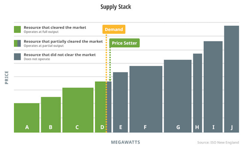
Here is a picture of how this works, from a market operator in the northeast (ISO New England). (1)
Source: ISO New England
In this case, plants A, B, and C are running at full capacity, and D at partial capacity. If more load came online, plant D would handle it. This would be evaluated every five minutes throughout the day, with micro-adjustments in between.
The emissions on the grid at the time shown above would be the average of A, B, C, and part of D. Because plants are chosen in order of lowest price, which is also lowest emissions, the average emissions will be relatively low.
The “marginal emissions” are the emissions that would come online if new load were added. In this case, the marginal emissions are those of power plant D. They are nearly always greater than the average emissions, and often by a considerable amount.
There are some exceptions to this “cheapest runs first” rule, which is why marginal emissions can sometimes be lower than average emissions. For example, some types of plants are less flexible and need to run throughout the day, and that includes many older and less efficient gas plants, as well as nuclear plants.
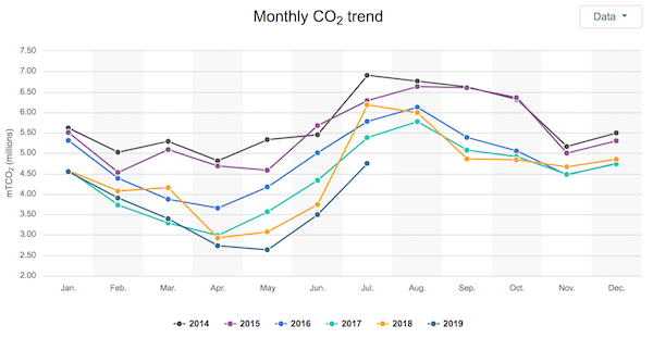
Average emissions are what we normally talk about and see on graphs like the one below, which shows CAISO’s emissions over time..
Source: CAISO
Marginal emissions are not as easily available for us to look at. They can be negligible on sunny, temperate days when we have more than enough solar (solar is on the margin). Or they can be up to 1400 pounds of CO2 per MWh on hot summer afternoons when we are forced to run our least efficient plants. Christy Lewis at WattTime gave me two data points that are a bit less intuitive. Let’s take them one at a time.
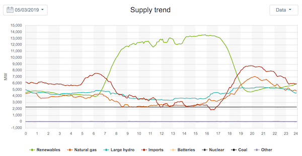
On a cool but sunny Friday afternoon, May 3 2019 at 1:27pm, average emissions were a low 284 lbs/MWh, but marginal emissions were a sky-high 1012 lbs/MWh. The graph below shows the power supply on that day.
Source: CAISO
Why were marginal emissions so high at 1:27pm? It is probably because a fast-acting but very inefficient “peaker plant” was activating. You can see a drop in solar and a rise in gas around that time, perhaps due to some persistent clouds over a large solar installation. That means the “peaker plants” would come online to cover the transient drop in solar.
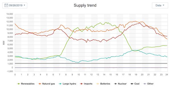
Here is the second data point. On a recent warm Thursday morning, September 26 2019 at 11:40am, average emissions were 626 lbs CO2 per MWh, while marginal emissions were 702 lbs/MWh. The graph below shows the power supply on that day.
Source: CAISO
You might wonder why the average was so high, given so much solar in the mix and marginal emissions indicating an efficient gas plant on the margin. Something much more inefficient than the marginal gas must be operating. It is possible we were running a less efficient and less flexible gas plant in order to prepare for a potential evening spike (it was a very warm day). Inflexible plants cannot ramp up quickly.
Marginal emissions are volatile and hard to predict. You can imagine that, if you have a flexible load, it is best to avoid times when marginal emissions are high. Since those times can be hard to guess, WattTime provides a platform that companies and organizations can use to schedule their load and lower their emissions. Using the right metrics to optimize load shifting really matters.
Here is a concrete example that shows how marginal emissions can be more accurate than average emissions for scheduling a flexible load. Suppose there are three power plants on the grid: 10 MW of solar (zero emissions), 10 MW of efficient gas (medium emissions), and 4 MW of inefficient gas (high emissions) that is brought on when demand is high. At 1am, demand is low, just 5 MW, so the efficient gas plant runs with room to spare. (Solar is not available at night, and this grid has no storage.) At 4pm, demand is much higher, 21 MW. The solar and medium gas plants are running at capacity, and the inefficient gas plant is at one-quarter capacity.
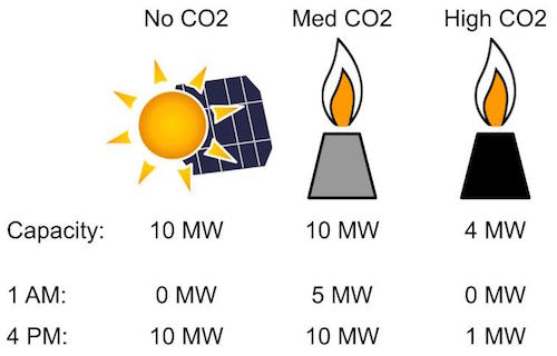
The average emissions are lower at 4pm, just over halfway between solar and the efficient gas. But the marginal emissions are lower at 1am. At 1am, new loads get served by the efficient gas plant, while at 4pm they get served by the inefficient gas plant. So it’s a good idea to move a 4pm load to 1am, at least as long as the 4pm load is high enough to engage that dirty plant. But it doesn’t make sense to move a 1am load to 4pm. It will just generate more emissions, though average emissions at that time are lower. Marginal emissions are great for optimizing load shifting, and flexible loads that are scheduled smartly like this help to reduce our emissions.
So all of this makes sense so far. But I’ve seen marginal emissions being used when I don’t think they make sense, so I checked in with Lena Perkins, the Manager for the Program for Emerging Technologies and acting Senior Resource Planner at the City of Palo Alto Utility. It turns out she shares that concern and helped me to think through the problem. She pointed out that marginal emissions are often short-lived and volatile, so while they are useful for short-term scheduling of flexible loads, they are not a good fit for evaluating longer-term changes. And because they reflect only the margin, they are also inapplicable for evaluating scenarios with very large loads, which may extend beyond the margin.
So it wouldn’t make sense to use marginal emissions to talk about carbon footprints or to talk about the impact of a new appliance. In fact, I struggle to find many good applications for marginal emissions beyond load shifting, though I’m still thinking this through. Let’s walk through a scenario involving adding a new electric appliance.
Suppose you have a grid with a 50 MW solar plant and a 100 MW gas plant. The typical demand is 100 MW, so the typical power would be half solar, half gas. The marginal power source is gas, meaning that any additional load would be matched with gas.
Now let’s say the homes in the area all have gas heaters. Residents can exchange them for $50 for electric heaters. If the electric heater is plugged into a 100% gas grid, its emissions are the same as the gas heater. But if the heater is plugged into a 50% gas grid, its emissions are one-half that of the gas heater. The electric heater has lower emissions than the gas heater as long as it is not running on 100% gas.
The residents are all concerned about global warming. You might think that they would rush to exchange their gas heaters for electric ones, since the grid is generally only half gas. But the residents are worried about marginal emissions, so they do no such thing. Plugging the heaters into the grid would only fire up the gas plants more, they reason. The heaters would generate the same emissions, plus it would cost them $50. The residents have somehow internalized that, even though the plugs in their houses all connect to the same “half gas” grid, any *new* electric appliance will actually be plugged into an “all gas” grid.
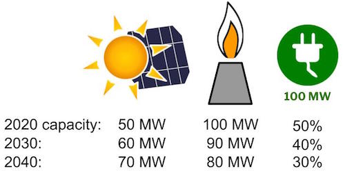
Even as the grid gets cleaner over time -- after 20 years, it is only 30% gas -- the residents cling to their gas heaters because they don’t want to plug into that marginal power source. (Of course by then the electric heater company has gone out of business.) Not until the grid has virtually no gas on it do these residents plan to switch over and reap the benefits of the clean supply.
What is wrong with this picture? It makes little sense imo to reason that the clean parts of the grid are allocated only to certain appliances, or that improvements to the grid accrue only to “old” appliances. Marginal emissions are short-lived and volatile, and should not be used to evaluate longer-term changes like this.
Unfortunately, there is some lack of agreement around which emissions model to use for which purposes, and Lena Perkins says that this can make the metrics vulnerable to “cherry picking”, when people use the metric that makes their initiative look most compelling. Consider efficiency improvements. Suppose you want to insulate your house or buy a new refrigerator. For the same reason that new additions to the grid should use average emissions, I believe that these removals from the grid should use average emissions as well, even though that makes the case for them weaker than if marginal emissions were used. But I’ve seen some policy makers suggest using marginal emissions for these initiatives.
Well, you know better now! From my perspective, anyway, it makes sense to default to average emissions for most things but to use marginal emissions to optimize short-term load-shifting. And hopefully we can drive both metrics down with aggressive policies that encourage more renewables to be built, more flexible demand to be developed, cleaner and cheaper storage technologies to come to market, and smarter load-shifting to eliminate dirty peaks. California is at the forefront of much of this, and it is fantastic to live here and support the people and organizations who are making this happen.
Notes and References
0. If you are interested in learning more about fuel switching, Palo Alto Utilities is hosting the Bay Area Electrification Expo on Thursday, October 10 from 2-7pm. There will be speakers and hands-on exhibits for residents and builders.
1. In states that use coal, for example, price and emissions are not aligned since coal is relatively cheap but has very high emissions.
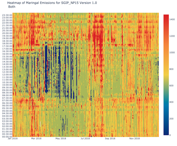
2. If you are interested in what marginal emissions look like, below is a heat map of marginal emissions for 2018 for the northern portion of CAISO (NP15), provided by Christy Lewis of WattTime. (These marginal emissions were calculated using the standard heat rate model for marginal emissions.) The bottom x-axis shows month of the year, from January on the left to December on the right. And the left y-axis shows hour of the day, from midnight and very early morning at the bottom to 11:30pm at the top. You can see that marginal emissions are generally lowest at midday and in spring, and highest in the evenings and late summer.
Current Climate Data (August 2019)
Global impacts, US impacts, CO2 metric, Climate dashboard (updated annually)
Comment Guidelines
I hope that your contributions will be an important part of this blog. To keep the discussion productive, please adhere to these guidelines, or your comment may be moderated:
- Avoid disrespectful, disparaging, snide, angry, or ad hominem comments.
- Stay fact-based, and provide references (esp links) as helpful.
- Stay on topic.
- In general, maintain this as a welcoming space for all readers.


